ترسیم توابع و منحنی های تراز در متلب

ترسیم توابع دو متغیره و سه متغیره و منحنی های تراز

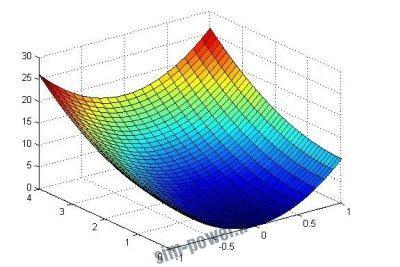
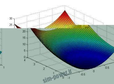
ترسيم توابع عددي دو متغيره

> x=-1:.1:1;
>> y=0:.1:4;

>> [X,Y]=meshgrid(x,y);
>> f=inline(’10*x.^2+y.^2′,’x’,’y’)
f =
Inline function:
f(x,y) = 10*x.^2+y.^2
>> surf(X,Y,f(X,Y))

– راه كوتاه : ابتدا محدوده صفحه X-Y را در corners وارد مي كنيم.

>> clear
>> f=inline(’10*x.^2+y.^2′,’x’,’y’)
f =
Inline function:
f(x,y) = 10*x.^2+y.^2
>> corners=[-1 1 0 4];
>> qsurf(f,corners)

ملاحظه مي گردد كه mesh بندي دقيقتر است.

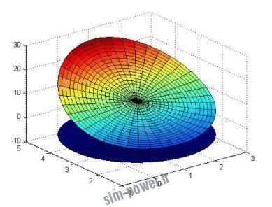
ترسيم توابع دو متغيره با مختصات قطبي

>> %first make a meshgrid in r,theta-coordinates
>> r=linspace(0,2,21);
>> thetta=linspace(0,2*pi,41);
>> [R,TH]=meshgrid(r,thetta);
>> %now convert into a curvlinear
>> X=1+R.*cos(TH);
>> Y=3+R.*sin(TH);
>> Z=X-1+Y.^2;
>> surf(X,Y,Z)
>> %add the plane Z=-5
>> hold on
>> surf(X,Y,-5+0*Z)
>> hold off

>> r=linspace(0,1,21);
>> thetta=linspace(0,2*pi,41);
>> [R,TH]=meshgrid(r,thetta);
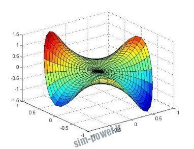
>> X=R.*cos(TH);
>> Y=R.*sin(TH);
>> Z=0.5*R.*sin(TH)+R.^3.*cos(3*TH);
>> surf(X,Y,Z)

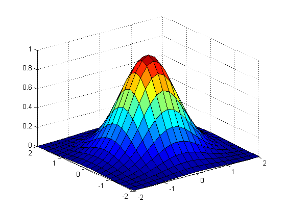
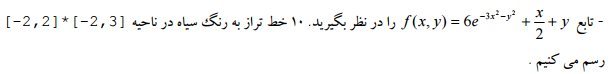
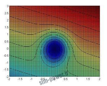
منحنيهاي تراز

>> x=-2:.05:2;
>> y=-2:.05:3;
>> [X,Y]=meshgrid(x,y);
>> f=inline(‘-6*exp(-3*x.^2-y.^2)+.5*x+y’,’x’,’y’);
>> Z=f(X,Y);
>> pcolor(X,Y,Z)
>> hold on
>> contour(X,Y,Z,10,’k’)
>> hold off

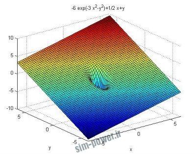
تكنيك رسم سريع توابع دو متغيره

تابع بالا را رسم ميكنيم:

> syms x y
>> f=-6*exp(-3*x^2-y^2)+.5*x+y;
>> ezsurf(f)

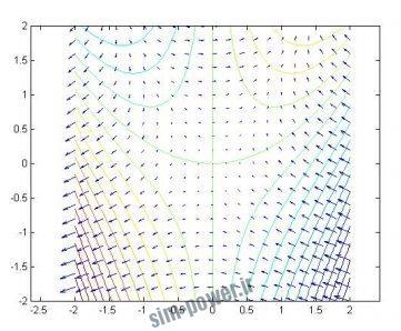
رسم بردار گراديان و منحني تراز

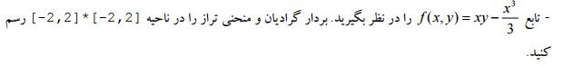
>> f=inline(‘x.*y-(x.^3)/3′,’x’,’y’);
>> fx=inline(‘y-x.^2′,’x’,’y’);
>> fy=inline(‘x’,’x’,’y’);
>> x=-2:0.05:2;
>> y=x;
>> [X,Y]=meshgrid(x,y);
>> Z=f(X,Y);
>> levels=[-6:0.5:6];
>> contour(X,Y,Z,levels)
>> hold on
>> xx=-2:0.2:2;
>> yy=xx;
>> [XX,YY]=meshgrid(xx,yy);
>> U=fx(XX,YY);
>> V=fy(XX,YY);
>> quiver(XX,YY,U,V)
>> axis equal

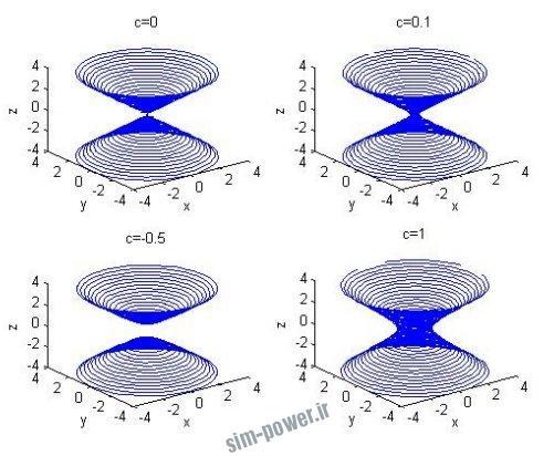
رسم سطوح تراز توابع سه متغيره

همان طور كه مي دانيم معادله سطوح تراز به صورت f(x,y,z)=c مي باشد. اين ترسيم به كمك M-File اي
به صورت (impl(f,corners,c انجام مي شود.

> f=inline(‘x.^2+y.^2-z.^2′,’x’,’y’,’z’);
>> corners=[-4 4 -4 4 -4 4];
>> subplot(2,2,1)
>> impl(f,corners,0)
ans =
The max over this domain is 32.00000
ans =
The min over this domain is -16.00000
>> subplot(2,2,2)
>> impl(f,corners,0.1)
ans =

The max over this domain is 32.00000
ans =
The min over this domain is -16.00000
>> subplot(2,2,3)
>> impl(f,corners,-0.5)
ans =
The max over this domain is 32.00000
ans =
The min over this domain is -16.00000
>> subplot(2,2,4)
>> impl(f,corners,1)
ans =
The max over this domain is 32.00000
ans =
The min over this domain is -16.00000

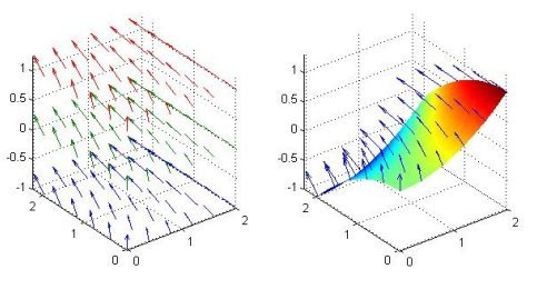
ترسيم ميدان برداري گراديان

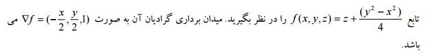
> [X,Y]=meshgrid(0:0.4:2);
>> U=-X/2;
>> V=Y/2;
>> W=1+0*X;
>> subplot(1,2,1)
>> for z=[-1,0,1]
Z=z+0*X;
quiver3(X,Y,Z,U,V,W)
hold on
end
>> axis image
>> %plot the surface
>> [XX,YY]=meshgrid(0:0.05:2);
>> ZZ=0.25*(XX.^2-YY.^2);
>> subplot(1,2,2)
>> surf(XX,YY,ZZ)
>> shading interp
>> hold on

> %add the gradint vector
>> Z=0.25*(X.^2-Y.^2);
>> quiver3(X,Y,Z,U,V,W)
>> axis image